Lane Finding from Video Feeds

February 23, 2017

Finding Lane Lines on the Road

The github repository with the associate IPython Notebook can be found here.

Objective

The ultimate goal of this project was to be able to identify lane lines in both images and videos. Namely, to develop a pipeline that utilizes different computer vision techniques to mark the location of lane lines. The approach that I took explored multiple techniques to obtain the best results:

Color selection with OpenCV with different color maps
- Grayscale
- Hue, saturation, and light
Gaussian blur to reduce noise
Canny edge detection
Hough line transformation
Moving average of previous lane lines

Color Manipulation

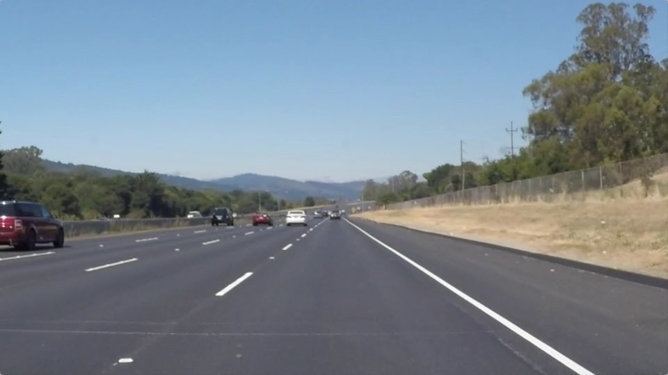
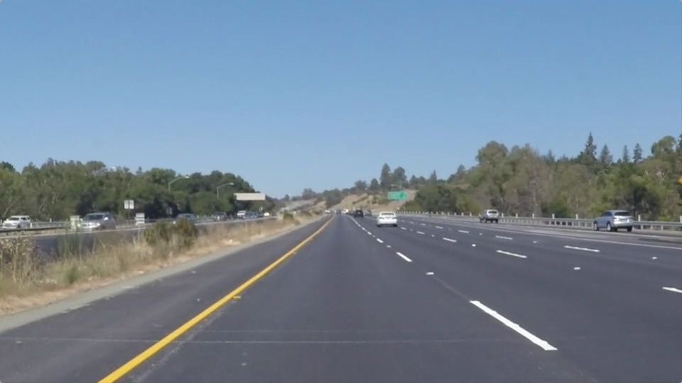
To start with, images came as screenshots from an onboard video feed.

lane1 lane2

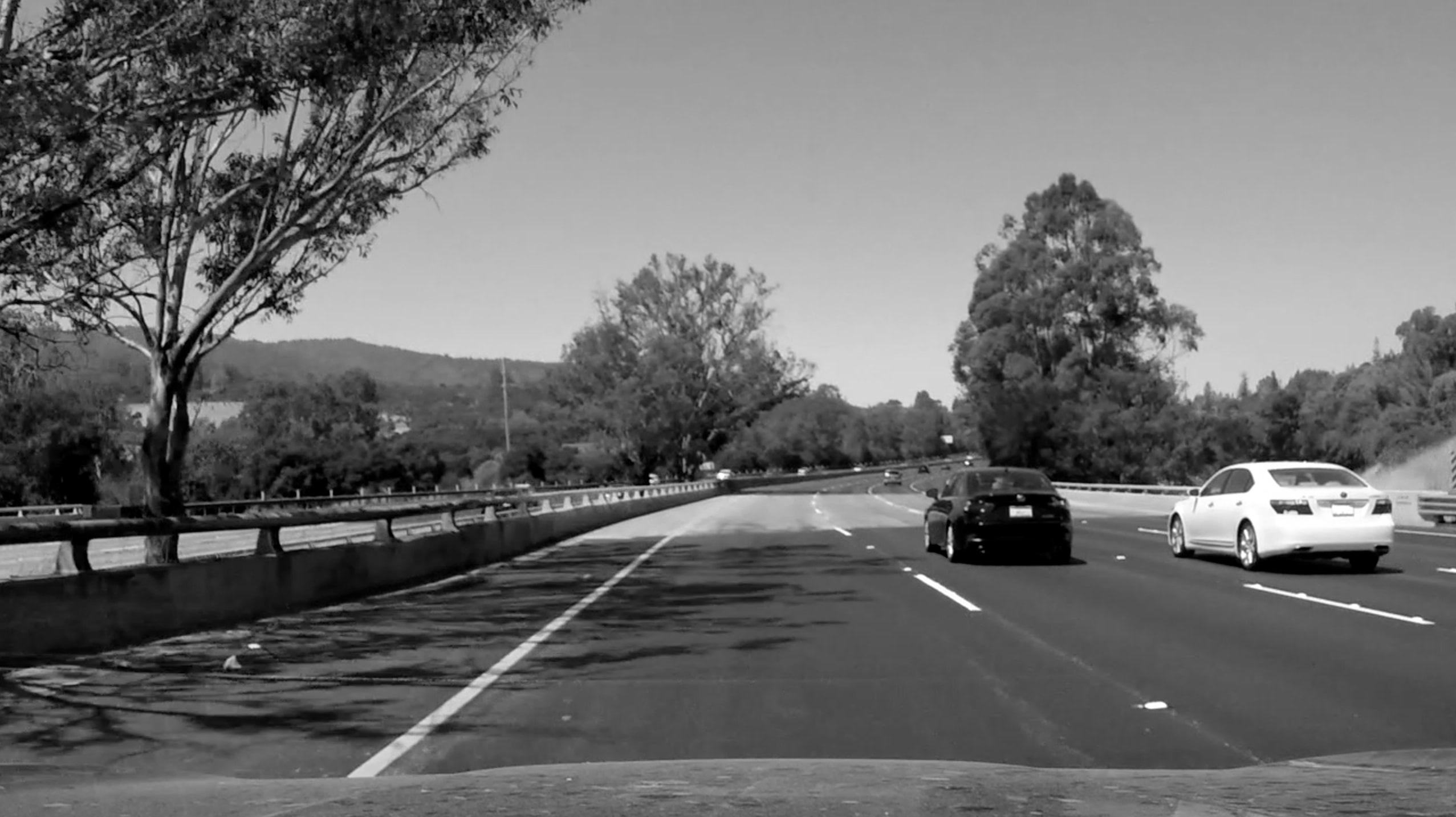
The first step that I took was to turn the image to grayscale to make it easier to work, namely to reduce the number of channels to work with. However, when dealing with more challenging images such as lane lines that are on non-contrasting backgrounds (white or gray tarmac), the eventual pipeline for lane linea detection does not perform well. In order to improve the performance, I switched to using hue, saturation, and light color space, which is better able to highlight the yellow and white lane lines.

Grayscale gray

HSL color space hsl

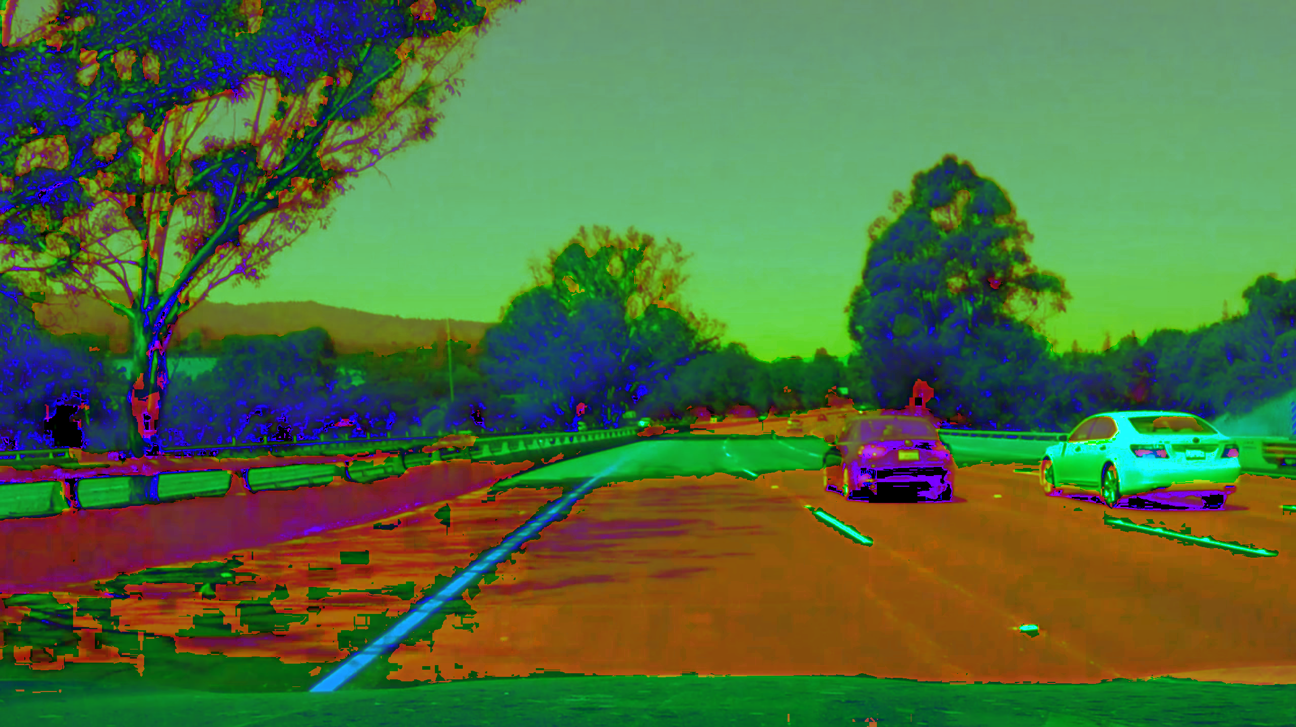
In the above image, we can see that the yellow lane is very clearly highlighted and the white line markings are also captured well when compared to the grayscale image. However, to further improve the performance of the processing pipeline, we can also select out the colors that we know we care about (in this case the yellow and white lines, which are now blue and green)

## color selection for yellow and white, using the HSL color space
def color_selection(image):

    hls_image = cv2.cvtColor(image, cv2.COLOR_RGB2HLS)

    white_color = cv2.inRange(hls_image, np.uint8([20,200,0]), np.uint8([255,255,255])) ## note that OpenCV uses BGR not RGB
    yellow_color = cv2.inRange(hls_image, np.uint8([10,50,100]), np.uint8([100,255,255]))

    combined_color_images = cv2.bitwise_or(white_color, yellow_color)
    return cv2.bitwise_and(image, image, mask = combined_color_images)

In the above code, I first convert the color map from RGB to HSL. Then I use the inRange function provided by OpenCV to select colors that fall into the white and yellow ranges. After that I combine the white and yellow masks together with the bitwise_or function.

With the above HSL image, we can now try to isolate the yellow and the white lines. While there are many different techniques that can be utilized here, I chose to detect the edges within the image using the Canny edge detection algorithm.

Edge Detection

HSL color selection hsl

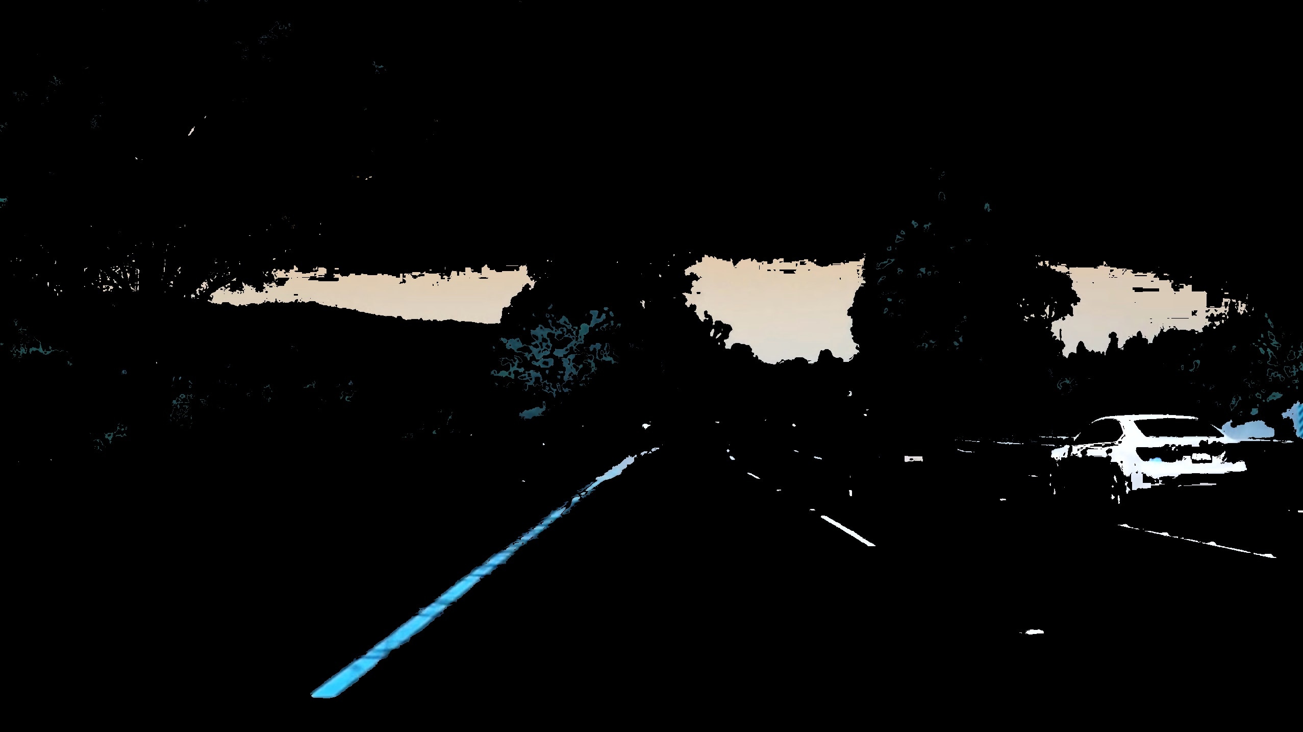
Given the above image, the goal is to pick out the lane lines. In order to do this, I use the canny edge detector algorithm. In short, the algorithm:

1. Applies a gaussian filter to the image to reduce noise
2. Finds the gradients in both the horizontal and vertical directions
3. Non-maximum supression, which is a way to thin the detected edges by only keeping the maximum gradient values and setting others to 0
4. Determining potential edges by checking against a threshold 
5. Finish cleaning potential edges by checking in the potential edge is connected to an actual edge

While, the canny edge detector automatically applies gaussian blur, I applied gaussian blur outside of the edge detector so that I could have more freedom with the kernel parameter. After running the image through the blurring and edge detection functions, the image is as follows. Note, the input image to this is the HSL color converted image.

HSL color selection with canny edge detection hsl_canny

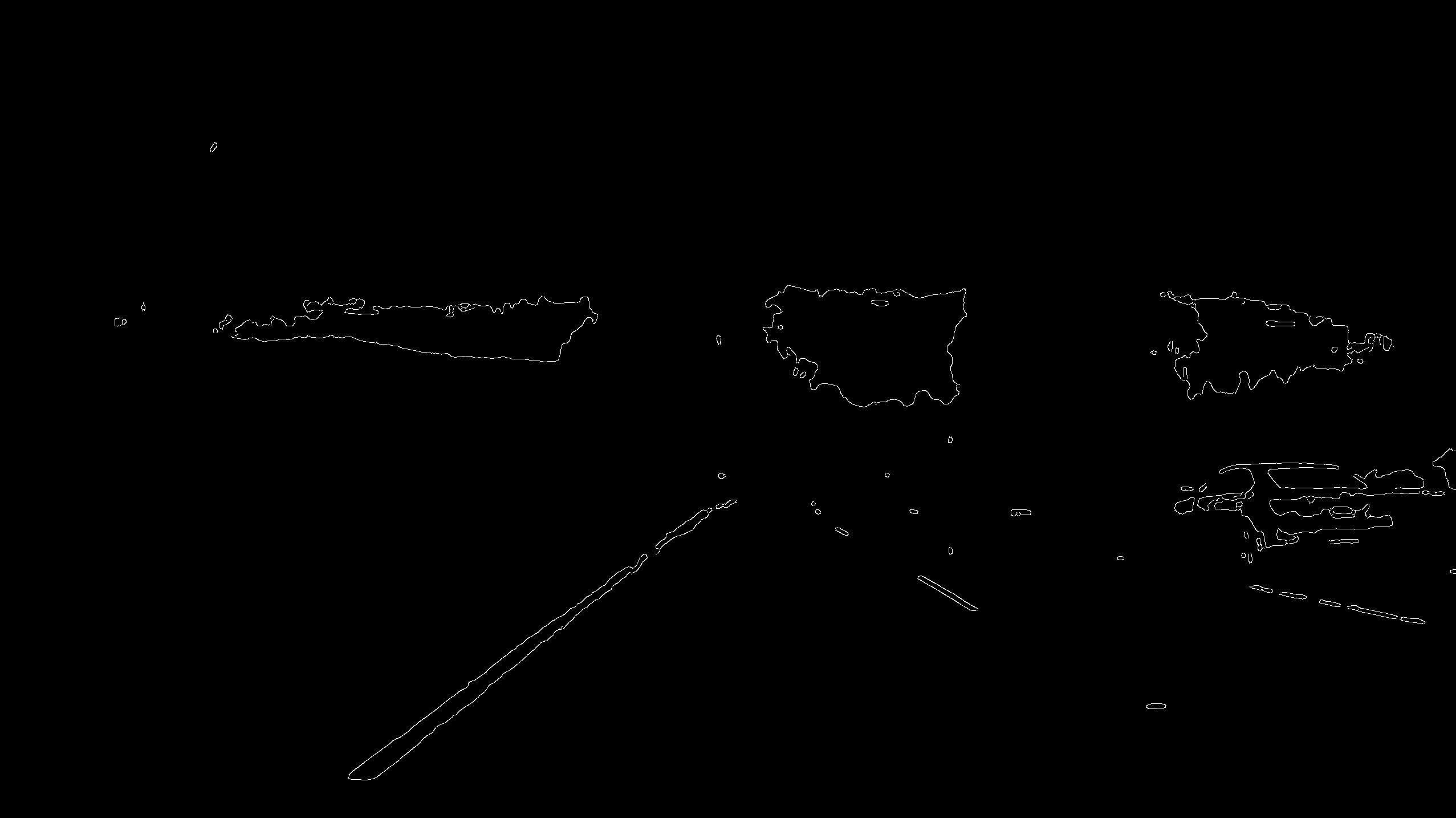
With the image above, we see that the lane lines are pretty well identified. It took a bit of trial and error to find suitable thresholds for the canny edge detector though the creator John Canny recommended a ratio of 1:2 or 1:3 for the low vs. high threshold. Although the image above seems to mark the lane lines quite well, there is still a lot of noise surrounding the lane that we do not care about. In order to address this, we can apply a region mask to just keep the area that we know contains the lane lines.

Region masking region_bounds

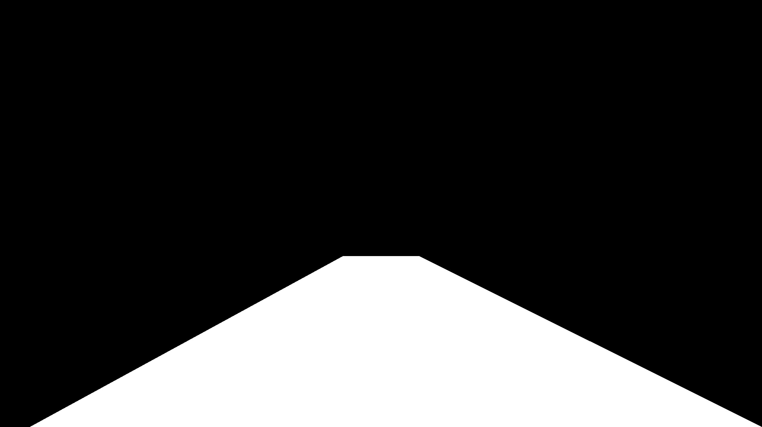
After applying the mask to the canny image, we get the following output. We can contrast this with the gray image after canny edge detection and the region selection.

Grayscale image with canny edge detection and region masking region_canny_gray

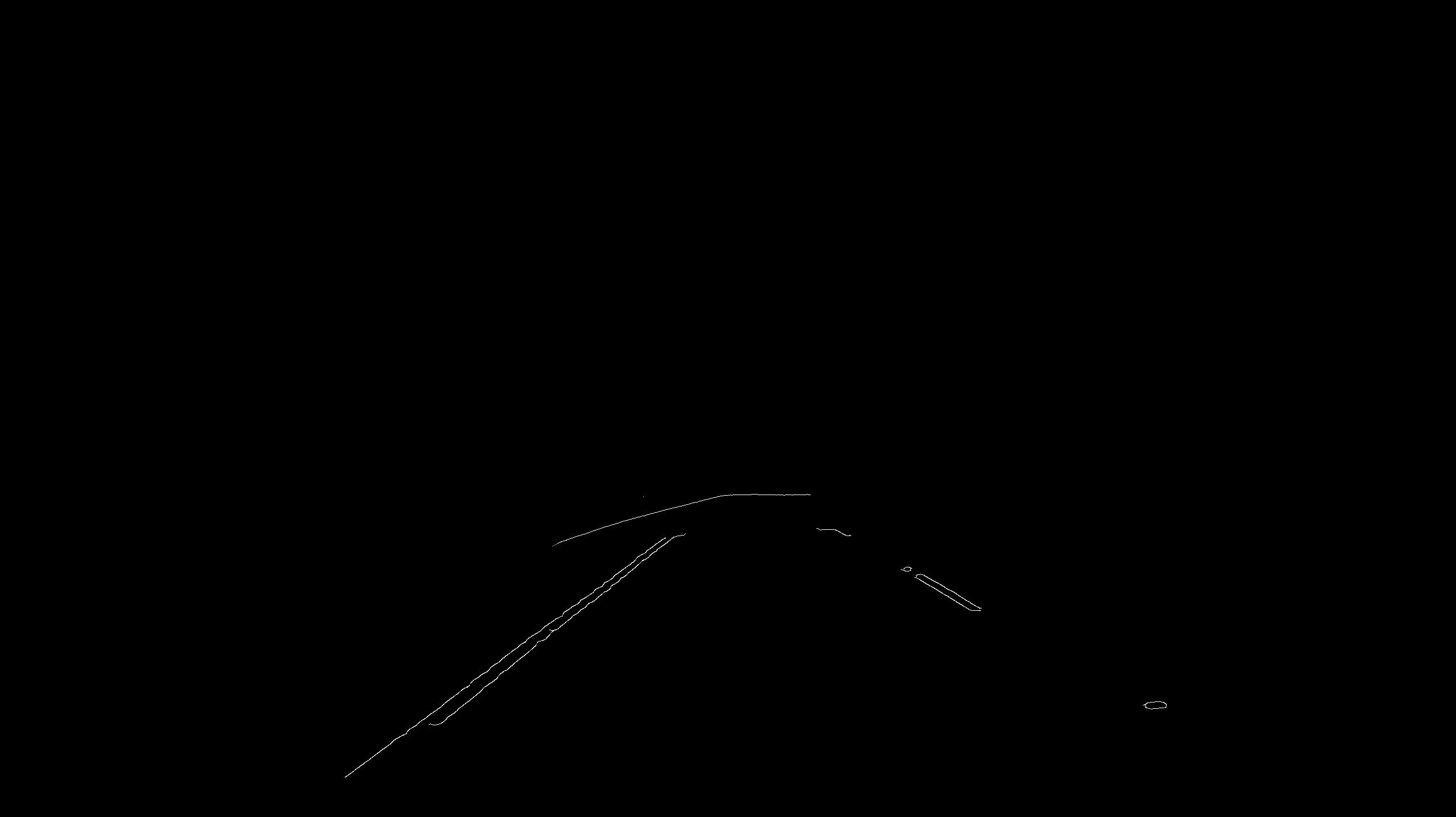
HSL color selection with canny edge detection and region masking region_canny

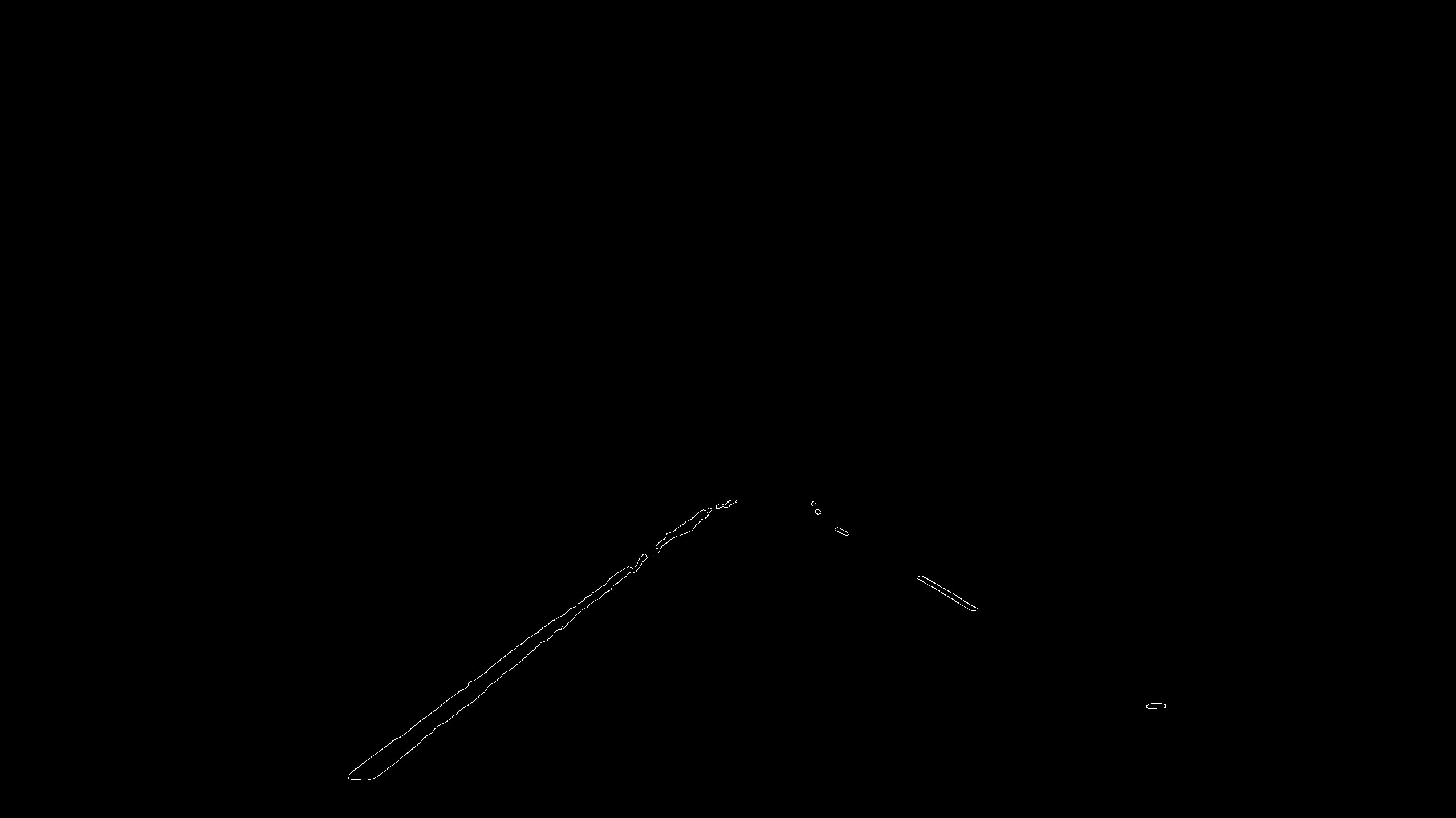
As shown above, the HSL version provides a cleaner indication of the lane lines. Below are the functions used in processing the images.

def canny(img, low_threshold, high_threshold):
    """Applies the Canny transform"""
    return cv2.Canny(img, low_threshold, high_threshold)

def gaussian_blur(img, kernel_size):
    """Applies a Gaussian Noise kernel"""
    return cv2.GaussianBlur(img, (kernel_size, kernel_size), 0)

def region_of_interest(img, vertices):
    """
    Applies an image mask.

    Only keeps the region of the image defined by the polygon
    formed from `vertices`. The rest of the image is set to black.
    """
    #defining a blank mask to start with
    mask = np.zeros_like(img)   

    #defining a 3 channel or 1 channel color to fill the mask with depending on the input image
    if len(img.shape) > 2:
        channel_count = img.shape[2]  # i.e. 3 or 4 depending on your image
        ignore_mask_color = (255,) * channel_count
    else:
        ignore_mask_color = 255

    #filling pixels inside the polygon defined by "vertices" with the fill color    
    cv2.fillPoly(mask, vertices, ignore_mask_color)

    #returning the image only where mask pixels are nonzero
    masked_image = cv2.bitwise_and(img, mask)
    return masked_image

Hough Line Transform

Now that we have a collection of edges, we need to identify the lane lines within the image. The hough line transform, which was first invented to identify lines within images, is great for this task. To learn more about this algorithm, this blog is a great resource.

_HSL color selection with canny edge detection, region masking, and hough transform hsl_hough

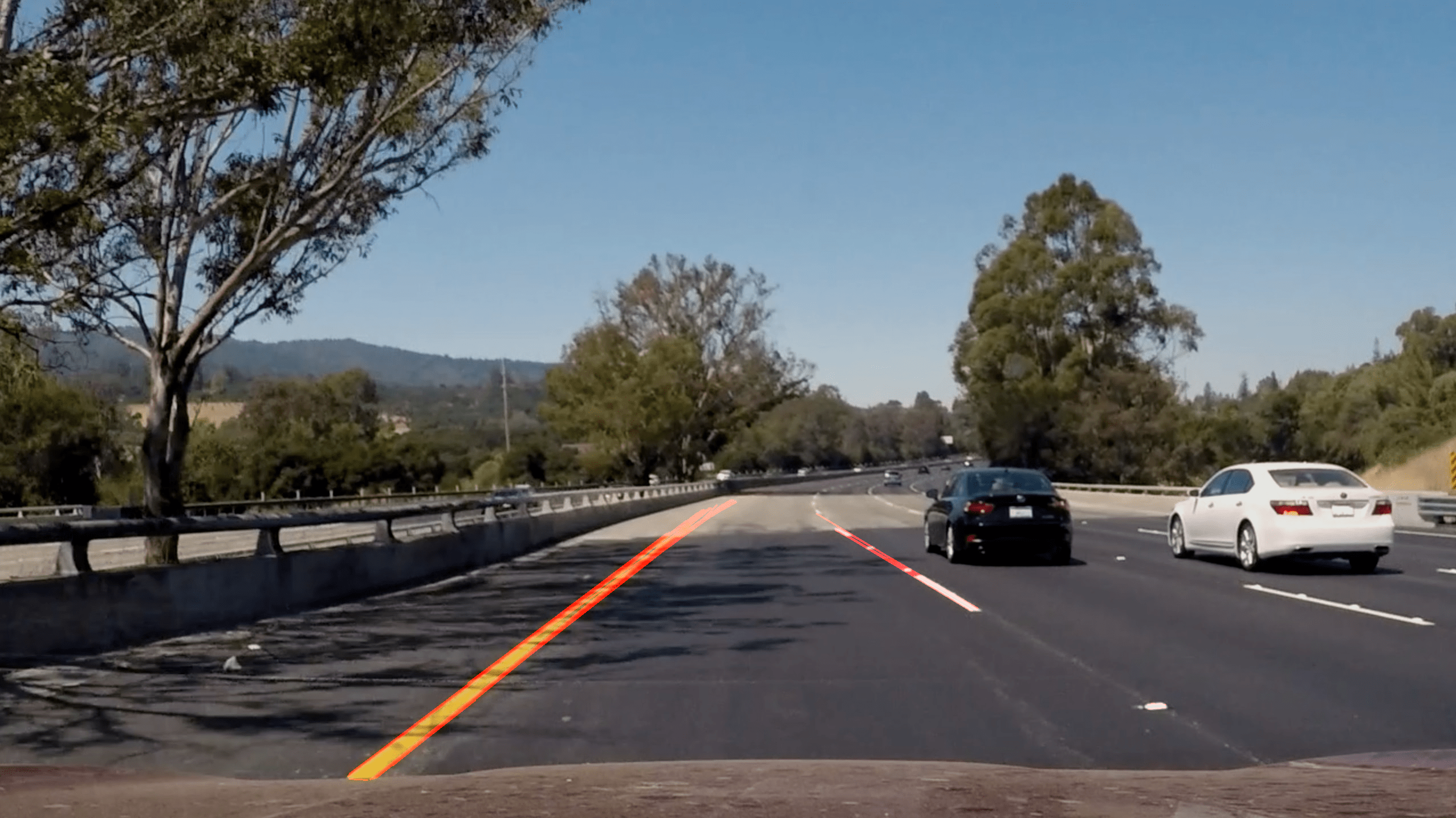
Pretty awesome! The lane lines have now been highlighted and boxed with the red lines. There are quite a few parameters that needed to be adjusted, but after adjusting the parameters, the algorithm is able to pick out the lines quite well. Note that the OpenCV version of the hough transform that we are using is the probabilistic version, which is an improvement over the original. In the IPython notebook, I use a different version of the hough_lines function that simple outputs the lines as a vector rather than overlaying the lines over the initial image.

Given the above image and specifically the hough lines, we now have a vector of multiple lines segments in the form of (x1,y1,x2,y2) endpoints. In order to draw lines on an image, we need a way to extrapolate an average line from the vector of endpoints.

def hough_lines_overlay(img, rho, theta, threshold, min_line_len, max_line_gap):
    """
    `img` should be the output of a Canny transform.

    Returns an image with hough lines drawn.
    """
    lines = cv2.HoughLinesP(img, rho, theta, threshold, np.array([]), minLineLength=min_line_len, maxLineGap=max_line_gap)
    line_img = np.zeros((img.shape[0], img.shape[1], 3), dtype=np.uint8)
    draw_lines(line_img, lines)
    return line_img

Lane Line Averaging

In order to find the average line on each side of the lane, we can first calculate the slope of each line segment and separate the positive and negative sloped lines, which represents the left and right lane lines. Then we can find the average of the left and right slopes and intercepts to get an average of the lanes. When I initially did this, the average was quite sensitive to outliers. I tried to adjust for the outliers by removing points that were greater than 1.5 standard deviations from the rest of the slopes. However, the averaged lines were still quite sensitive to the outliers.

Ultimately, by calculating the line length and calculating the weighted average of the lane line, the output was much more stable and robust against spurious line segments that the hough transform identified.

def avg_lines(lines):

    neg = np.empty([1,3])
    pos = np.empty([1,3])

    ## calculate slopes for each line to identify the positive and negative lines
    for line in lines:
        for x1,y1,x2,y2 in line:
            slope = (y2-y1)/(x2-x1)
            intercept = y1 - slope*x1
            line_length = np.sqrt((y2-y1)**2+(x2-x1)**2)
            if slope < 0 and line_length > 10:
                neg = np.append(neg,np.array([[slope, intercept, line_length]]),axis = 0)
            elif slope > 0 and line_length > 10:
                pos = np.append(pos,np.array([[slope, intercept, line_length]]),axis = 0)

    ## just keep the observations with slopes with 2 std dev
    neg = neg[to_keep_index(neg[:,0])]
    pos = pos[to_keep_index(pos[:,0])]

    ## weighted average of the slopes and intercepts based on the length of the line segment
    neg_lines = np.dot(neg[1:,2],neg[1:,:2])/np.sum(neg[1:,2]) if len(neg[1:,2]) > 0 else None
    pos_lines = np.dot(pos[1:,2],pos[1:,:2])/np.sum(pos[1:,2]) if len(pos[1:,2]) > 0 else None

    return neg_lines, pos_lines

## removing the outliers (adapted from http://stackoverflow.com/questions/11686720/is-there-a-numpy-builtin-to-reject-outliers-from-a-list)
def to_keep_index(obs, std=1.5):
    return np.array(abs(obs - np.mean(obs)) < std*np.std(obs))

The above function calculates the slope, intercept, and line length of each line segment. At this point, we can take the average lane lines from the above function and plot the lane lines onto the original image.

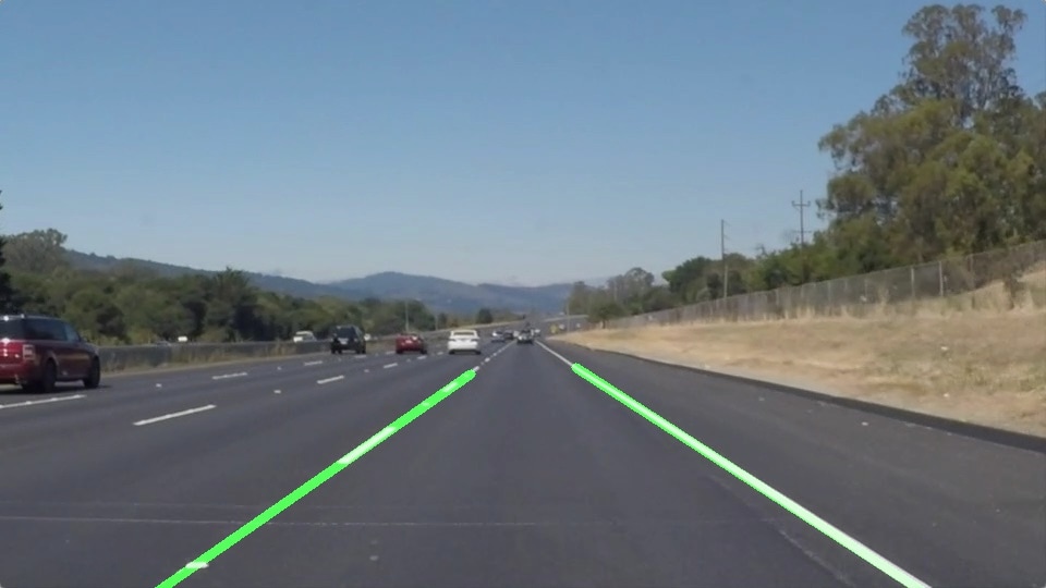
Final processed image hsl_final

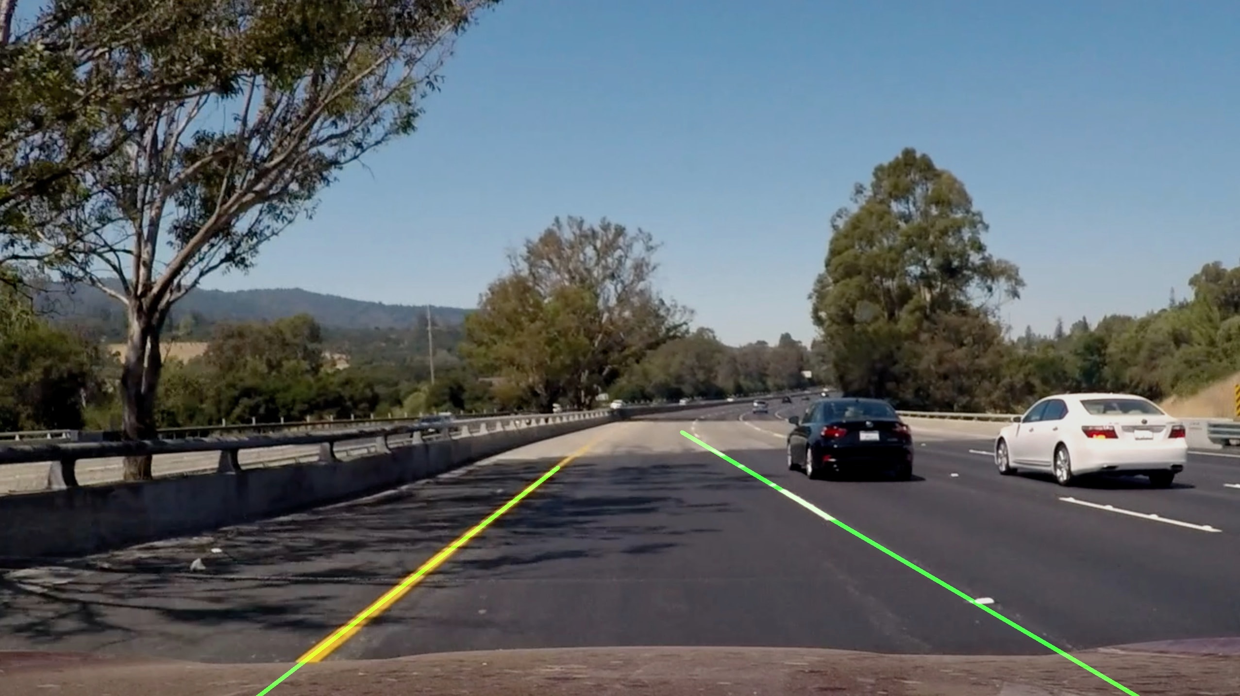
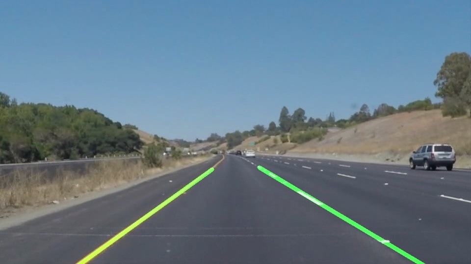
It seems to have performed quite well! Below are a few other sample images of the outputs from the lane finding pipeline.

Sample processed images solid_yellow solid_white

Applying Lane Finding to Videos

Now that we can identify and mark the lane lines within the image supplied, we can use the algorithm on a video, which is just a sequence of images. If we just apply the pipeline directly to the video, we get the following.

Lane Finding (Without Previous Averaging)

The video seems to show the lane lines without any problems, but when we take a closer look the lane line highlights are jittering and jumping across back and forth around the actual location of the lane line. While, the algorithm basically accomplishes the problem that we first set out to solve, maybe we can improve on this.

Specifically, the lane lines coming from a video feed usually do not change dramatically from second to second. If we take this into account, we can "smooth" the lane lines plotted out by keeping a queue. With each frame of the video, we can pop off the oldest set of lane line endpoints. Then for all the remaining lane lines and the newest lane line, we take an average to get the "smoothed" lane line.

Below is the code for the lane line detector and the link to the test videos.

The above videos show that the new detector with the lane line averaging works quite nicely! Although if there are drastic changes the algorithm does not follow those changes until a bit later, we can fiddle with this by changing the size of the queue.

class lane_detector:
    def __init__(self):
        self.prev_lane_lines = []

    def find_mean_lines(self, lane_lines, prev_lane_lines):

        ## add the new lane line
        if lane_lines is not None:
            prev_lane_lines.append(lane_lines)

        ## only keep the 10 most recent lane lines
        if len(prev_lane_lines) >= 10:
            prev_lane_lines.pop(0)

        ## take the average of the past lane lines and the new ones
        if len(prev_lane_lines) > 0:
            return np.mean(prev_lane_lines, axis = 0, dtype=np.int)

    def pipeline(self, image):
        imshape = image.shape

        ## selecting yellow and white colors
        color_selected_img = color_selection(image)

        ## Define a kernel size and apply Gaussian smoothing
        kernel_size = 17
        blur_img = cv2.GaussianBlur(color_selected_img,(kernel_size, kernel_size),0)

        ## apply canny edge detection
        canny_img = canny(blur_img, low_threshold= 50, high_threshold=160)

        ## apply region of interest
        vertices = np.array([[(100,imshape[0]),(imshape[1]*.45, imshape[0]*0.6), (imshape[1]*.55, imshape[0]*0.6), (imshape[1],imshape[0])]], dtype=np.int32)
        region_img = region_of_interest(canny_img, vertices=vertices)

        ## apply hough transformation
        rho = 1 # distance resolution in pixels of the Hough grid
        theta = np.pi/180 # angular resolution in radians of the Hough grid
        threshold = 15 # minimum number of votes (intersections in Hough grid cell)
        min_line_len = 25 #minimum number of pixels making up a line
        max_line_gap = 250   # maximum gap in pixels between connectable line segments

        lines = hough_lines(region_img, rho, theta, threshold, min_line_len, max_line_gap)

        ## get the average slopes and intercepts for each lane line
        slopes_intercepts = avg_lines(lines)

        # find the endpoints given the slopes and intercepts
        endpoints = gen_endpoints(image, slopes_intercepts)

        ## generate lane lines on a black image
        lane_lines = gen_lane_lines(image, endpoints=self.find_mean_lines(endpoints, self.prev_lane_lines))

        final_img = weighted_img(lane_lines, image)

        return final_img

Shortcomings & Next Steps

While the detector works fairly well for straight roads, there are limitations:

Curved Roads
Lane markings that are not yellow or white
Different perspective

In order to deal with these shortcomings, we would need to make the algorithm more robust to differences in the input video. For example, to deal with the curves in the road instead of setting a fixed length for the lane line highlights, which is currently 60% of the image height, we might be able to use the length of the identified line segment from th hough line transform as a proxy for how long the highlight should be.

The yellow and white lane lines might be harder to deal with, but we can combine human input as well as computational methods. For example, if there are training images from roads in different areas with different colored markings, we can keep a "dictionary" of these lane colors and setup the algorithm to look for the colors that expected given the geographic region in consideration.

The videos that were supplied as test videos were all basically filmed at the same angle and the roads were also fairly similar. However, if the vehicle was traveling over a hill or out of a trough the perspective would change. In these cases, the algorithm might not perform as well. In order to adjust for this, we can first apply a perspective normalization to the input video so that input would always have the same orientation and perspective.

Overall, this project was interesting and fun! It incorporated a lot of techniques and concepts that have been available for many years, but is now being applied to interesting problems like self-driving cars.

Posted on: February 23 2017

Category: Python