August 16, 2017

In this project, the main goal was to use computer vision and machine learning techniques to identify and track vehicles in images and video feeds. Also, take a look at the Jupyter Notebook for more details. Check out the final video output here.

Specifically, the project consisted of the following steps:

• Perform a Histogram of Oriented Gradients (HOG) feature extraction on a labeled training set of images and train Linear SVM and Random Forest classifiers to compare the performance differences
• Apply a color transform and append binned color features, as well as histograms of color, and append to your HOG feature vector
• Normalize the features and randomize a selection for training and testing
• Implement a sliding-window technique and use the trained classifier to search for vehicles in images
• Run the pipeline on a video stream and create a heat map of recurring detections frame by frame to reject outliers and follow detected vehicles
• Estimate a bounding box for vehicles detected

Getting Started

There are many features that we can consider extracting from an image or a video frame. We can first take a look at the images that we have in the training set (vehicles images can be found here and non-vehicle images can be found here) from to get a sense for what might work well. The images are compiled from both the GTI vehicle image database and the KITTI vision benchmark suite. In addition to the data mentioned, I also supplemented the training data with labeled images from CrowdAI. This added about ~60k images of vehicles (both front and rear of the vehicle).

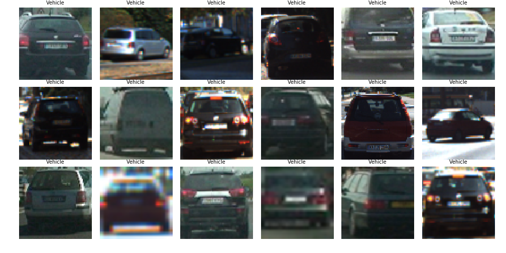
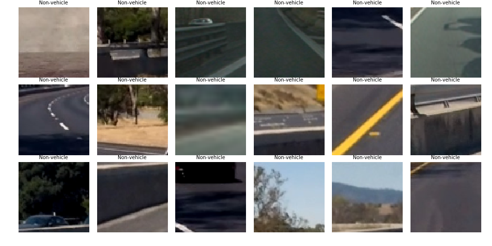
Very clearly, there are images of vehicles and non-vehicles. The object is to see if we can train a machine learning algorithm to distinguish the feaures of vehicles.

As expected, the images above show cars are various zooms, crops, and angles while the non-vehicle images show scenes do not contain any cars. We can use these images to extract relevant features, which will ultimately be used to train our classifier.

Extracting Features

Histogram of Gradients (HOG), Spatial Binning, and

First, we can try to extract the histogram of gradients. The gradients of an image will help to identify the structures within the image. On the otherhand, if we use color, it might be difficult to extract the relavant features because the same model car can be different colors. The gradient is able to capture the edges of the shape of the car. We use a modified version that averages the gradients across multiple cells to account for some possible noise in the image.

Specifically, we can use the scikit-image implementation of the HOG extraction function. There are a couple of parameters that we had to adjust to get meaningful features:

• orientations: represents the number of orientation bins that the gradient information will be split up into in the histogram
• pixels_per_cell: specifies the cell size over which each gradient histogram is computed
• cells_per_block: specifies the local area over which the histogram counts in a given cell will be normalized

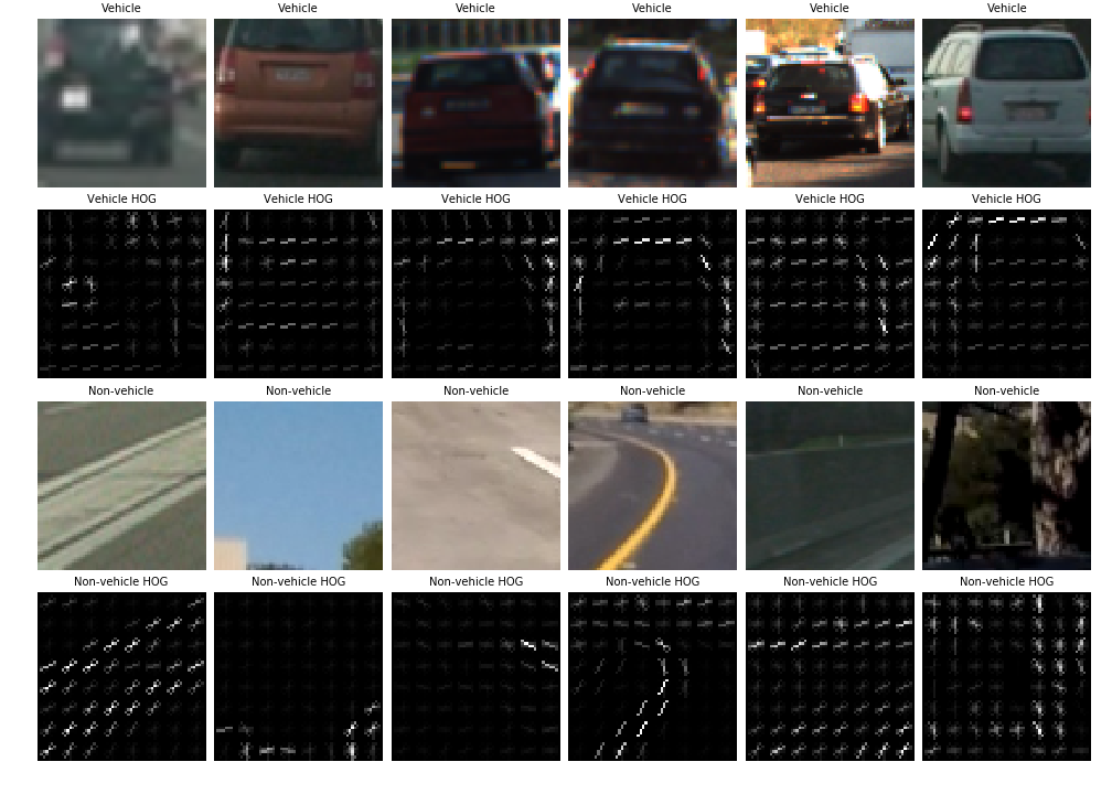
Awesome, we can look closely at the HOG visualizations and see that the gradients seem to capture the shape of the vehicles quite well. If we compare the HOG visualizations of the vehicles vs. the non-vehicles, we can see that there is a difference between the different types of images.

In order to find suitable values for the various parameters, we can approach the problem as a feature engineering problem and use cross validation in the model evaluation step to gauge which parameters work best. Next, we can explore another set of features: color.

Color Histogram

We can imagine that there are different shaped histograms if we look at different colored cars. However, if we go one level deeper and use a color space that is able to differentiate between cars and non-cars, this would be even more helpful in the feature space. Specifically, in some cases the vehicles are usually more saturated when compared to a pale background. In the end after trying different color spaces, the LUV color space ended up performing the best when evaluated using cross validation (note that there are many other features in the feature set.

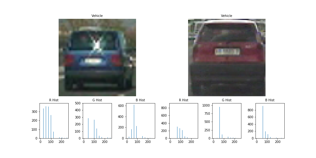
The above example used the typical RGB color space, but the model was trained using images converted to the LUV color space.

Spatial Binning

We can also take into account the raw pixel values. However, there might be too many features if we do that so we can reduce the size of the image to return a slightly lower resolution image with the same features.

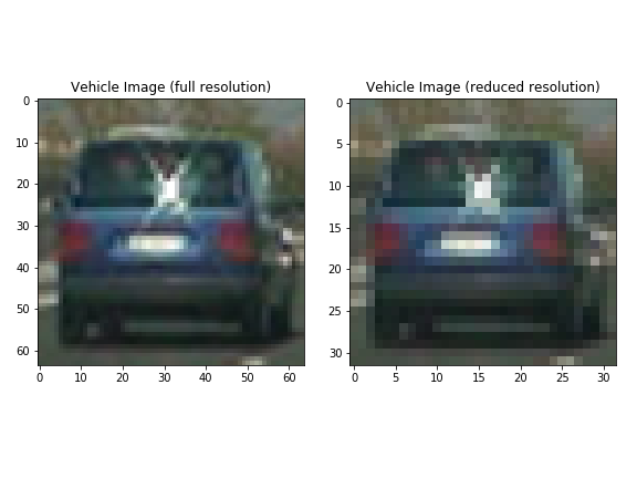
We can see that in the above image the vehicle image on the right has a lower resolution but still captures most of the information that we see in the original image.

At this point we have quite a few techniques to extract both color and gradient information from the images. We can define a pipeline to extract these features. Note that if and when we combine the color and gradient features we need to normalize and scale the features so that the different scales of the features do not adversely affect the classifier that we will build.

The final set of parameters used in the various feature extraction methods are listed below:

Parameter	Value
Color Space	LUV
Orientations	8
Pixels per Cell	8
Cells per Block	2
HOG Channel	0
Spatial Bin Size	16
# of Color Bins	32

Classification

With the features extracted, we can build a classfier to identify whether the object in the image is a vehicle or not. The details and the code for this section can be found in the Jupyter Notebook.

To start with, we can use a Support Vector Machine Classifier, which is fairly quick and accurate when it comes to the features that we extracted. The final Linear SVM model achieved an accuracy of 98.36% without significant parameter tuning. However, in the end we used a Random Forest model that was optimized using grid search over the various parameters to achieve a performance of 99.39% on the test set.

With slightly more time we could have further refined the model; however, the model wa already performing fairly well. Beyond tuning the parameters using grid search, the CrowdAI image data set also helped boost the performance of the model.

Sliding Window Search

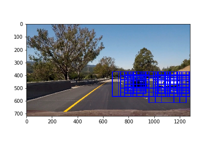
Now that the classifier can identify if an image or a frame of a video contains a car, we need to find a way to look through the image to search for potential car matches so that we can run it against our classfier. One idea is to use a sliding window approach to scan through the image to identify possible car-like objects, then pass it to our classifier.

The above image shows the different scale windows that we use to identify cars. Note that the image above shows windows that are overlapping so there are actually many more windows that we are searching through. Each of the windows represents a snapshot that then gets passed through to the classifier. The 3 different images above show different scales because a closer car is larger while a farther car is smaller. The different scales help to capture cars wherever they are in the image.

After running each of the windows through a classifier, we are able to identify the windows where a vehicle is present.

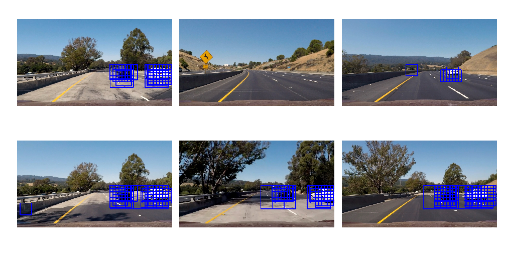
Cool! It seems like the classifier works fairly well. It was able to pick up where the cars are in each of the test images. However, beyond just the obvious cars there are also some incorrect classifications. Furthermore, while the above described method works and performs fairly well, it is slow because it reruns the HOG extraction every time there is a new window.

A better implementation would run the HOG extraction once and reuse the extracted data by "sliding" a window across the initially extracted matrix. The below images show the output of this improved implementation.

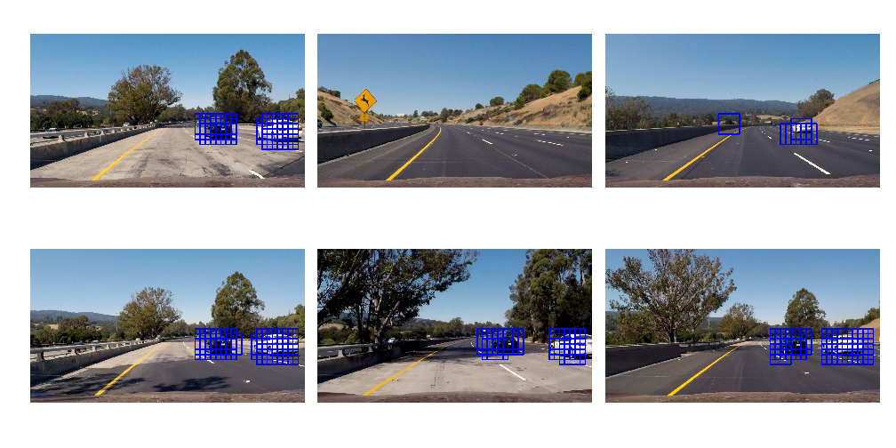
In order to deal with the false positives, we can count the number of times that a pixel is contained within a bounding box and use that to create a heatmap of which pixels are most likely to be of a vehicle.

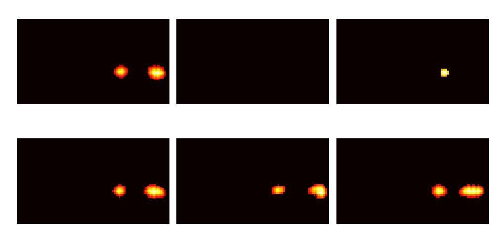
The heatmap strategy works fairly well to control for the noise in our images. Now, we can use the scipy label function to identify where the non-zero observations or the 'heated' observations are.

The image of the left shows the final output with the hotspots surrounded by a bounding box. The image on the right shows the heatmap of which pixels are contained within the most windows. Bringing this all together we can now identify the areas where a vehicle is most likely to be.

When applying this pipeline to videos, we need to deal with jitter that is introduced frame to frame. In some cases the pipeline might not be able to identify a vehicle in the frame. One method for dealing with this is to store a history of the bounding boxes. Then, for each frame we can run a heatmap of the bounding boxes to get a smoother version of the bounding boxes. Ultimately, this step along with the heatmap creation mentioned above helps in accounting for false positives, because the final output is an average of the last couple of frames.

Discussion

Overall, this project was quite interesting and required techniques from both computer vision and machine learning. It was a joy to finally see the algorithm identify cars in the video feed. However, there were definitely challenges and there is room for improvement.

• Performance: One of the major drawbacks of the current pipeline is that it is relatively slow. Even though the classification of the frame is quick, the extraction of the features is slow. An improvement to the speed of the extraction could mean that this pipeline could be applied to an actual real-time feed. Currently the rate of feature extraction and classification is roughly 1.5 frames per second.
• Noise: Although the current pipeline does a fairly good job at identifying the cars, in some cases there are still misclassifications. Ideally these misclassifications need to be dealt with so that the classifications don't lead to our self-driving car crashing!
• Feature Extraction: The process of identifying the right features to extract is really difficult and we can actually imagine that using a convolutional neural network might help in extracting the relevant features. A CNN is able to identify features that are important without much supervision. This might perform better than explicitly setting up the pipeline to extract the HOG, color histogram, and raw pixel values. Additionally, a car that is oout of the ordinary would be an issue for this pipeline.