February 23, 2018

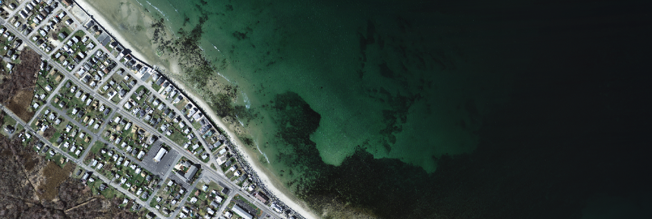
With the wealth of earth observation data made available by agencies such as NASA and ESA or private companies like DigitalGlobe and Planet Labs, there are a lot of interesting applications that can come from the combination of this data with recent advances in computer vision and machine learning. While the application of computational techniques to satellite imagery is not novel, development of techniques in this direction have the potential to impact many pressing social and humanitarian related causes.

One question of interest is how to make use of the available data to reduce dependence on limited resources. Namely, when considering rapidly growing cities it is important to understand the growth of the city not only in terms of numerically, but also it can be immensely helpful to have a geographical understanding of the city's development. For example, even if the city does not yet have paved roads, common paths or informal roadways are important to map out. While local surveyors could construct the most accurate representations, local communities might not have the resources to send surveyors out with any regularity. Instead, tools that make use of earth observations and modern computer vision techniques can serve as the first step of the process towards eventual verified and published maps.

Introduction

This post will focus mainly on road extraction using deep learning techniques given aerial imagery. The code repository contains the preprocessing notebook, model, and other utilities used in the project. The main training data comes from Volodymyr Mnih's PhD thesis. The data was mainly collected from Massachusetts roads and ground truth labels were created using rasterized OpenStreetMap data. Although there are many machine learning frameworks for creating models that can process satellite imagery, I use PyTorch mainly because I wanted to become familiar with the framework. On the modeling side, the main model considered is a form of fully convolutional network called UNet that was initially used for biomedical image segmentation.

Although PyTorch is relatively easy to use, it lacks some of the visualization and monitoring capabilities that Tensorflow has (through Tensorboard). I follow the efforts of other PyTorch users and use Tensorboard to monitor the training phase.

Data Gathering and Pre-processing

The main source of data for this project, as mentioned, is from Mnih's PhD thesis. In the future, it might make sense to use data from other sources to increase the robustness of the model and the overall size of the data set (for example, the SpaceNet Challenge data).

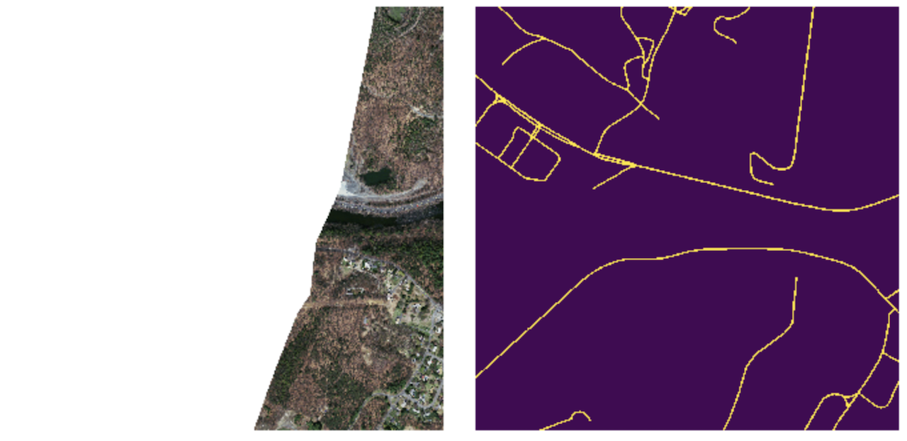
The Mnih road data consisted of 1171 satellite images of Massachussets, each of which were 1500x1500 pixels (specific details are in Chapter 6 of Mnih's thesis). The data was split into 1108 training images, 14 validation images, and 49 test images. During the augmentation stage, I first manually removed training images that had greater than ~50% of the image missing and ended up with 862 training images. I removed these examples so that the model would be less affected by examples that did not match with the ground truth labels. The image below has missing data, but the target map still shows all the road networks. In this case, the network would get penalized even though it does not have the image data to predict on.

Initially, I was unsure how to manipulate the input images so I resized images to ~768x768 pixels and further cropped images to ~300-400 pixels, but immediately I realized that the GPU I was using (Quadro P4000 with 8GB of memory), which comes with the Paperspace instance, did not have the memory to handle images of that size with a batch size greater than 3. Therefore, I directly rescaled images to ~256x256 pixels from the 1500 pixel images. Upon closer inspection, I realized that the ground truth roads, which were already relatively underrepresented, were even more sparse than before due to the rescaling. In the end, I randomly cropped 15 256x256 pixel images from each original image to retain the resolution as well as increase the training data set to 12916 images.

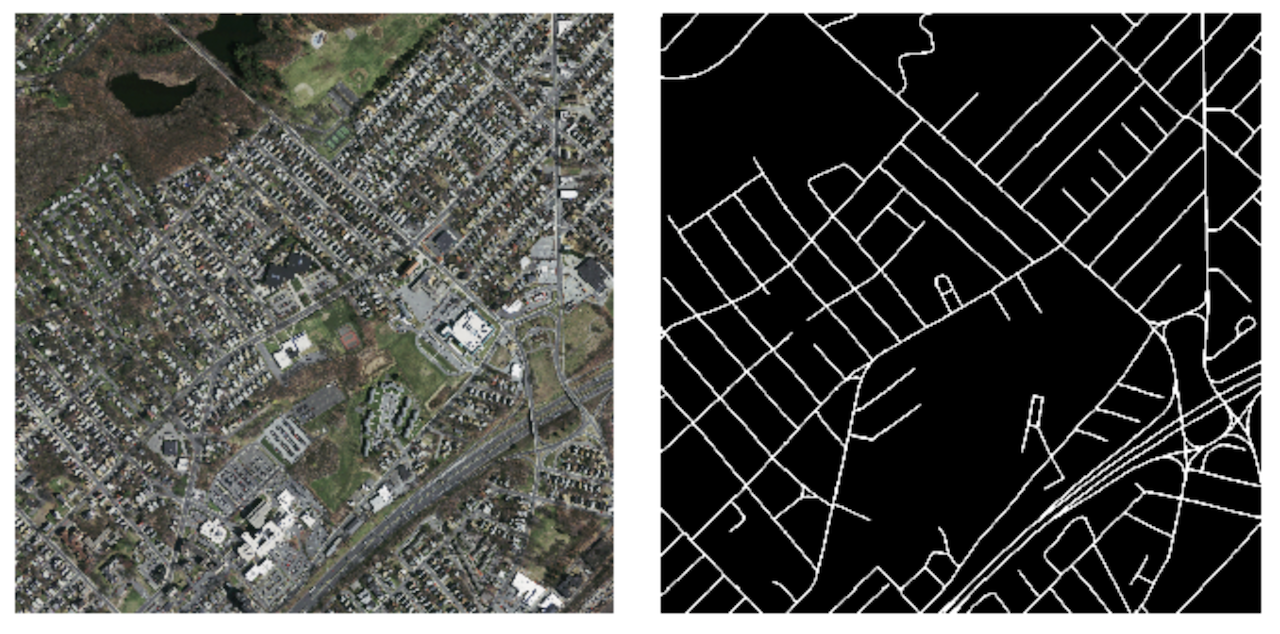
After creating the images, I loosely referenced this PyTorch data loading tutorial and created the data loader. One of the most time consuming parts of the process was figuring out how the transforms would operate on both the input images and the target maps. As opposed to other image classification tasks, the target map also needs the equivalent operation. I spent a lot of time working out the details for the data augmentation classes (thankfully PyTorch is flexible and there are lots of examples all around). However, in the end I ended up not using any of the transforms, except ToTensorTarget, which makes use of the PyTorch functional to_tensor transform because PyTorch expects tensors as input to the models.

Model Architecture, Training, and Parameter Tuning

Remote Compute Resource

When considering the different resources to use for the computation and training of the model, I considered AWS, Crestle, FloydHub, and Paperspace. Although I already had some AWS credits and had used AWS before, I heard good things about the other services and typically the compute was cheaper for comparable hardware. I wanted to give the other services a try and ended up choosing Paperspace because Fast.ai's Paperspace template made it really straight-forward to get started.

If you are considering different resources for personal projects or even for your team, here are some summary statistics about the different options!

Model Architecture

As mentioned above, the main architecture used in the project is related to the UNet architecture that was first proposed for biomedical image segmentation. I chose this specific architecture because it was simple enough to quickly code and also because I had read a lot about the successes of this particular model for satellite imagery and other semantic segmentation projects (see this deepsense.ai post). If you are interested in learning about some of the other architectures in the space, I enjoyed reading this blog post.

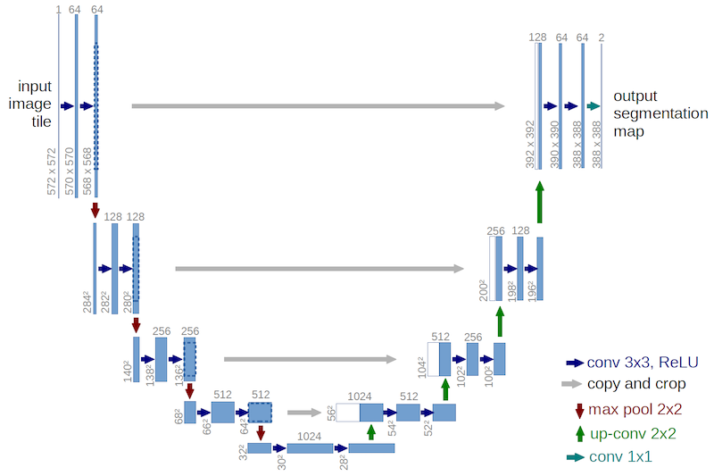
Compared to the original model structure shown above, there were some modifications that I made in order to work around the GPU memory limitations that I had. Namely, while the network still has the same number of layers, the number of trainable parameters is reduced to ~25% (~7.2 million) of the original network (~28.9 million).

While reviewing the original paper and other resources, I was unsure how the original author's were upsampling in the decoding portion of their network (probably because I skimmed too quickly...the implentation details are pretty clear in the image shown above...). Specifically, I was confused because in some places I saw bilinear upsampling and in other places I saw reference to deconvolution (transpose convolution or fractionally strided convolutions). In the end, I tested using transposed convolutions instead of bilinear upsampling and got worse results so ended up sticking with bilinear upsampling. I also tried nearest neighbor upsampling but did not get better results. Here are some resources that I went over to learn more about transposed convolutions (Types of Convolutions in Deep Learning and Deconvolution and Checkerboard Artifacts).

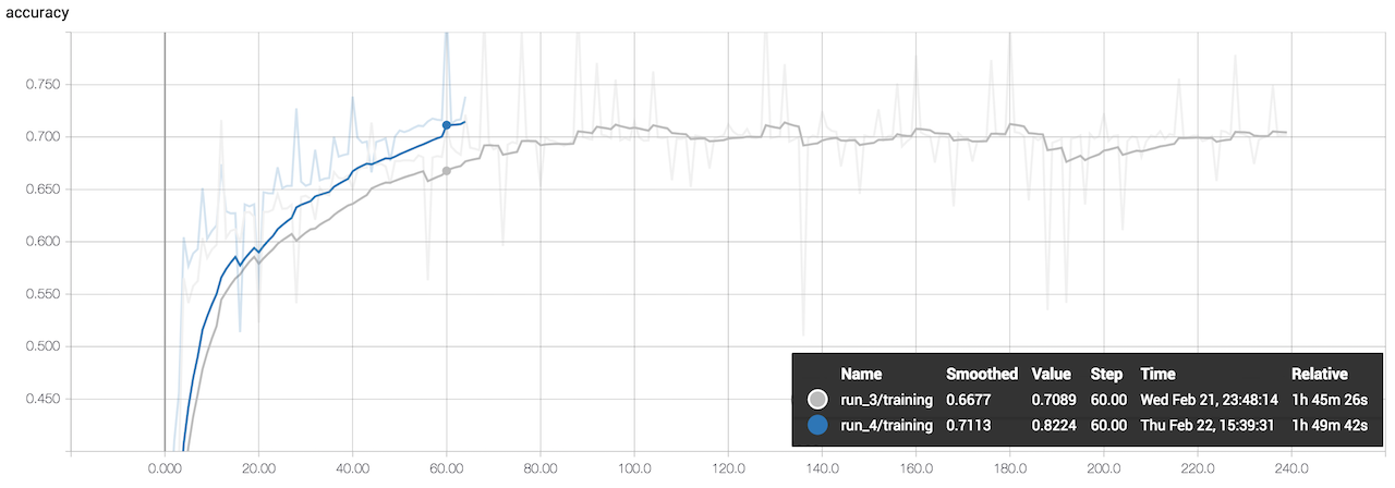
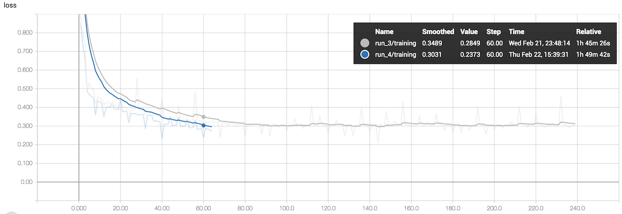
As I was monitoring the gradients of the network, I noticed that many of the gradients were very small if not zero; in other words, I was noticing vanishing gradients. This led me to change the activation function to exponential linear units (ELU) then parametric rectified linear units (PReLU) instead of rectified linear units (RELU) used in the original paper. The ELU activation helps with this problem and ultimately helps with convergence. I switched to PReLUs after noticing smoother training and also lower loss throughout the training process. When reading up on PReLU's it seems like not zeroing out the negative portion and adaptively learning the coefficient helps to improve accuracy (though these coefficients are additional parameters that need to be learned).

I also added batch normalization to the network at each step before the activation because it helps when randomly initializing the network (CS231n note on this). After doing some digging, I moved the batch normalization to after the activation because it led to better performance (I had a hard time finding papers to verify this...but in my experience training and validation loss was lower).

Loss Function and Learning Rate Scheduler

I settled on using binary cross entropy combined with DICE loss. Many previous implementations of networks for semantic segmentation use cross entropy and some form of intersection over union (like Jaccard), but it seemed like the DICE coefficient often resulted in better performance. By combining the two losses (similar approach with Jaccard instead of DICE in this paper), we can make use of both the probability of the correct prediction and the overlap between prediction and target. The accuracy that I used to monitor the training was the DICE coefficient.

When considering the learning rate, most of the papers that I referenced above used a learning rate of 0.001, which was then decreased with some step schedule. I experimented with different learning rates, schedulers, and step sizes (number of epochs in between the decrease), but the results often varied based on the optimizer that I used. For example, when using stochastic gradient descent (SGD) with Nesterov momentum I observed that starting with a learning rate greater than 0.005 for this particular problem often led to divergence. I ended up using the Adam optimizer with weight decay (1e-5 for regularization) and an initial learning rate of 0.001 that was decayed by 0.1 every 18 epochs. When I switched to using PReLU's I took out the weight decay, as mentioned in the PyTorch documentation, because the weight decay would affect the parameters that are being learned for the PReLU. One potential next step is to individually define the parameter groups to enable weight decay for the rest of the parameters except the PReLU parameters.

Monitoring Training Progress

While training the network, it became apparent that keeping an eye on the progress would dramatically reduce my stress levels. Mainly because I was paying for the compute and if the network diverged, it would be helpful to catch it sooner rather tnan later. As a result, I started looking around for options for monitoring the training and validation of the network. It turns out that since PyTorch does not have much support for visualization yet (since it is relatively new) many users have started to use Tensorboard to do the monitoring. I had heard about Tensorboard before but had never used it meaningfully. It was quite straight forward getting Tensorboard up and running (check out this tutorial). I mostly utilized the logger that was in the tutorial, but changed the data and the structure of the images that was being passed to the Tensorboard summary writer object.

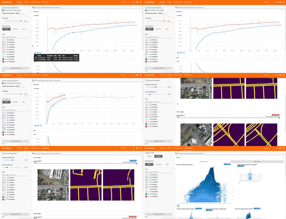
I found it helpful to be able to compare the target map and the predicted result. Tensorboard also kept track of the different runs so I could go back and toggle the previous runs to quickly compare how the new parameters affect the training.

I was able to learn a lot about the quality of the training data that the network was getting by looking at the Tensorboard summary images that I plotted. Because some of the aerial imagery may have been captured before (or after) the OpenStreetMap data, some roads that were marked in the target maps were no longer present in the aerial images (or the other way around). While I was afraid that this would impact the training, I figured that increasing the number of samples and increasing the batch size would reduce the effect that these discrepancies had on the network.

In the above example, the middle ground truth map has a driveway, which the prediction does not pick up. However, looking at the satellite image it is hard to tell if there really is a road there. In many other cases, driveways are not mapped as roads.

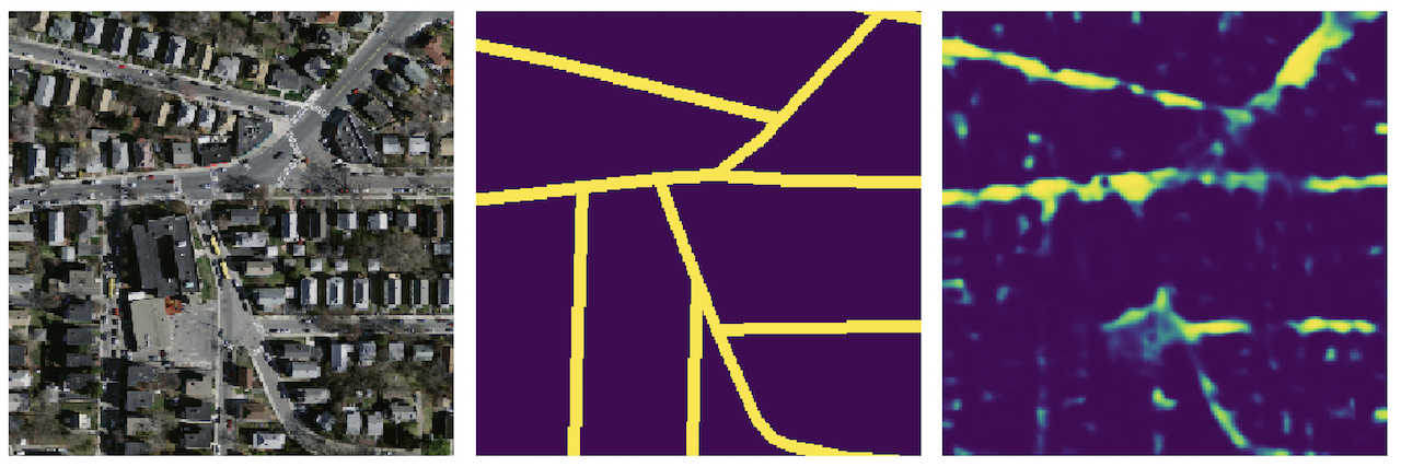
The above two images show the initial stages of the training process where the weights are being learned. It is interesting that the image before shows that the model identifies white and gray surfaces. Then, in the second example the network is beginning to identify the roads rather than the rest of the gray surfaces.

It is interesting to note that by the end the model is able to distinguish roads vs. other forms of pavement (like parking lots) that could easily have been mistaken as roadways. Though this creates an issue when the roads around parking lots are actually considered roads (as seen in the second test example below).

Results

Looking at the predictions above, some of the edges appear to be quite hazy. One potential solution is to threshold the output. Since the last step was to pass the output of the model through a sigmoid, all of the values are 0-1 so it represents probabilities. In the example below, the threshold value was set to 0.3. The output looks cleaner and the roads are better defined. In some of the blog posts related to the DSTL Satellite Imagery Feature Detection Kaggle competition as well as other semantic segmentation papers, researchers use conditional random fields (CRF) to do post-processing. This is a potential future step.

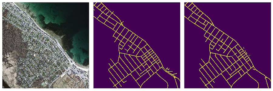
The example shown above is the full size image passed through the network. This result seems to be better than the result below because the roads are more "normal" and well defined. In the example below, there are some places where the roads seem to be part of the parking lot or other parks.

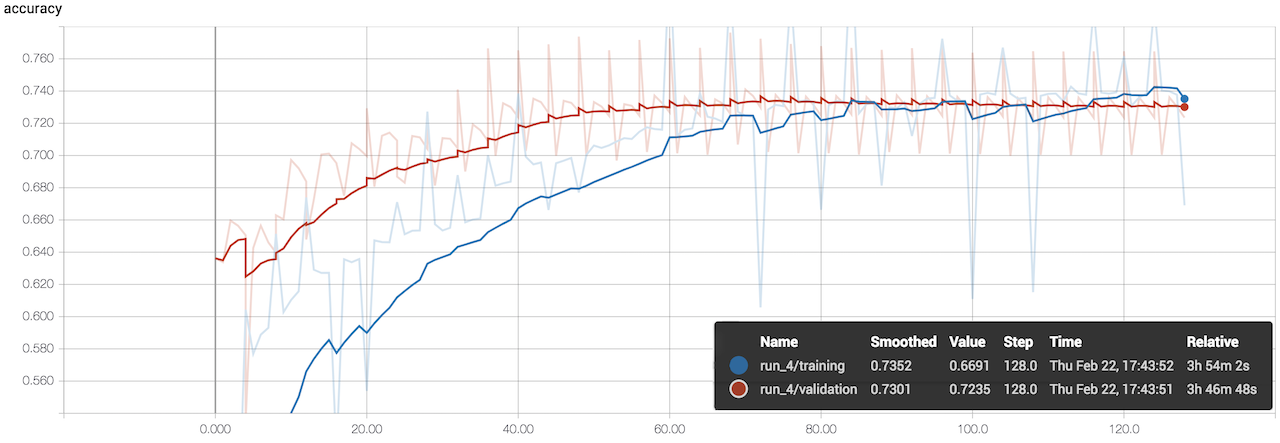
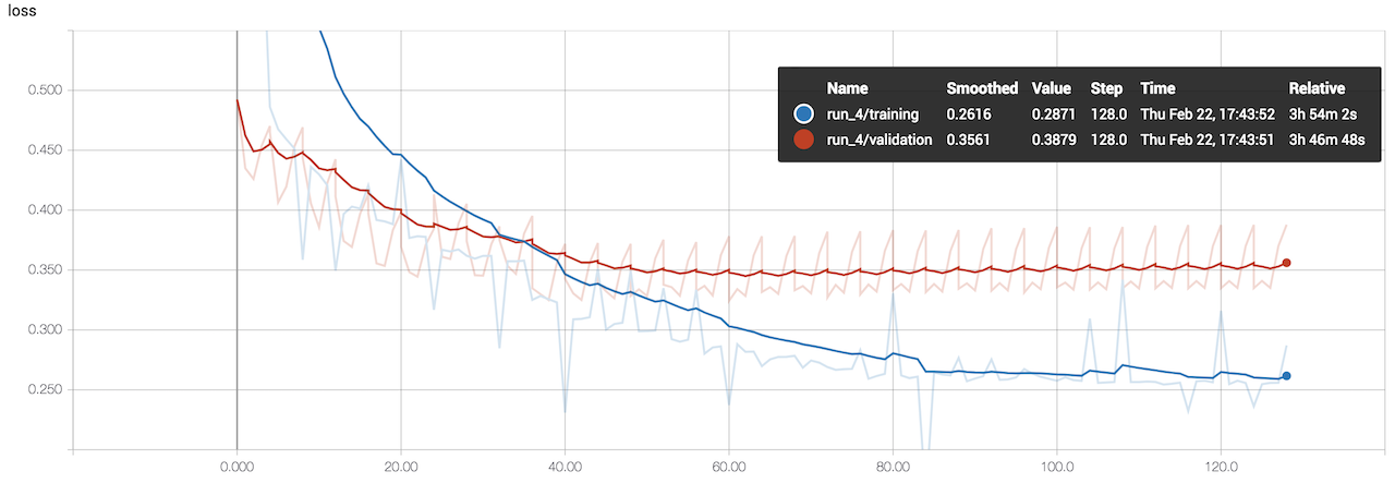
The final model reached a validation accuracy of ~0.73 (DICE coefficient) and a validation loss of ~0.35 (binary cross entropy loss combined with DICE loss)

Discussion and Next Steps

Overall, the network performed relatively well for the amount of time that it took to create and train. While the robustness of this solution might be challenged when predicting road networks in other areas, with a broad enough range of data it is reasonable to expect fairly good performance. One question that comes to mind is how the network will handle situations where roads are not paved. As shown in the interesting examples above, unpaved paths are not easily detected because the training data did not contain unpaved roads.

Beyond the above mentioned methods for possible improvements to the model, such as using CRF for post-processing or using additional data sources for more robust predictions, below are some other possibilities for next steps.

• Multispectral Images: One improvement would be to use multispectral images that capture wavelengths beyond the typical visible range. This is helpful because vegetation or cloud cover might obstruct roads and buildings, but other wavelengths capture the reflective properties of pavement or roads even when there are some obstructions.

• Pretrained Model Weights for Initialization: While training a network from scratch is possible, many top performing networks are typically pre-trained on ImageNet then fine-tuned on the specific data set at hand. Other transfer learning techniques also make the training process quicker and the eventual accuracy better. In the case of semantic segmentation, one possibility is to use a pre-trained network as the decoder and an untrained network as the encoder (as shown in this paper).

Ultimately, while this post details a technical solution, it is important to keep in mind that a purely technical solution often misses out on many important social aspects. Therefore, although technology can make it easier and more cost effective for certain tasks, it should be designed with input from the eventual end users.