March 28, 2017

In this project, we classify German traffic signs. The code for this project can be found in this IPython notebook.

The objective of this project is to ultimately design, train, and test a convolutional neural network (CNN) to see if we can accurately classify the traffic signs. Specifically, with image classification tasks the variability of input images might cause the model to perform poorly. In order to remedy this situation, we will consider preprocessing steps to ensure that the model is robust to varying input images. Furthermore, depending on how the model performs, we may need to consider regularization steps such as dropouts or L2 regularization.

To start with, I use the LeNet-5 architecture that was first published by Yann Lecun's lab in 1998. Eventually, I augmented the training set with rotated and zoomed images, normalized images, and included dropouts for the fully connected layers. This led to a final model that achieved ~95% on the validation set and ~94% on the test set.

Data Set Summary & Exploration

Before jumping into the model, we can take a look at some of the images within the dataset.

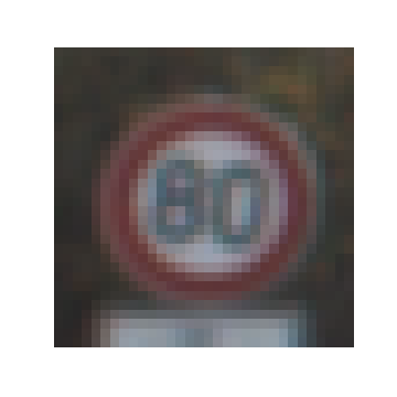
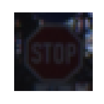
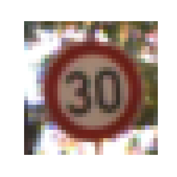
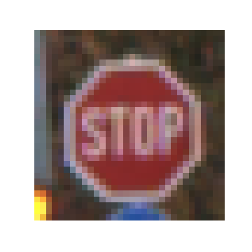
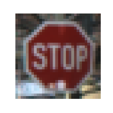
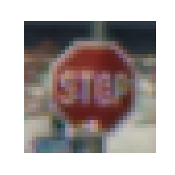
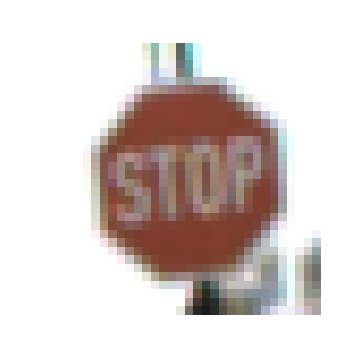
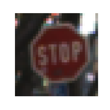
The images vary quite a lot in terms of brightness/ we can imagine that the orientation of the images might also be quite different. More specifically, we can take a look at just stop signs and see that there is quite a lot of variation.

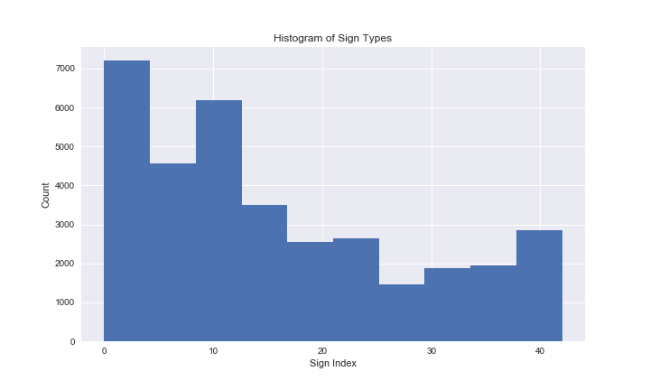
Additionally, we can take a look at how the traffic sign classes are distributed (to see if the classes are evenly balanced). Looking at the below histogram, it seems like there are some classes that are represented 7x as much as the least represented class. Later on we might want to upsample the less represented classes to make the model more robust.

Below are some summary statistics calculated from the dataset that we have:

• Number of training examples = 34799
• Number of validation examples = 4410
• Number of testing examples = 12630
• Image data shape = (32, 32)
• Number of classes = 43

Data Preprocessing and Model Evaluation

The input data is rather varied in terms of lighting and orientation of images. In order to improve the accuracy of the model, we can implement some preprocessing steps on our images.

Grayscaling, Mean Subtraction, and Normalization

First of all, I implemented grayscaling of the traffic sign images. While there may be some information lost because the color information in the image might contain information about the traffic sign, grayscaling simplifies the 3 channels into a single channel, which can lead to quicker model training. Additionally, taking away the color channels might allow the CNN to "focus" on extracting the important non-color features better.

After performing grayscaling, I performed mean subtraction and normalization of the image pixels. Specifically, in the cs231n course notes Andrej Karpathy mentions that the standard preprocessing techniques involve mean subtraction img = img - np.mean(img) and normalization img = img / np.std(img).

Before Processing Images

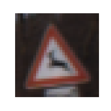
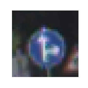
After Processing Images

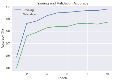
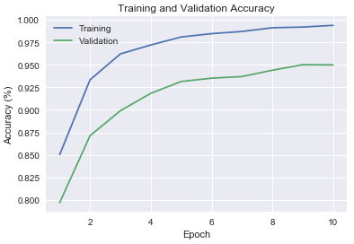
At this point, model performed fairly well and better than the 93% on the validation set that was required in the grading rubric. To start with, the original LeNet-5 network applied to the colored images achieved ~88% on the validation set. Then the gray scaling, mean subtraction, and normalization combined with dropouts on the fully connected layers pushed the validation accuracy to ~95%. - I added the dropouts because looking at the original train vs. validation curve, the model shows strong overfitting. As to why the drops were only applied to the fully connected layers, looking at this kaggle question the author mentions that we usualy do not apply dropouts to the convolution layer because the convolution layer is meant to extract features and also does not have that many features to regularize.

Original LeNet Architecture

LeNet Architecture with Grayscaling, Normalization, and Dropouts

Model Evaluation and Deep Dive

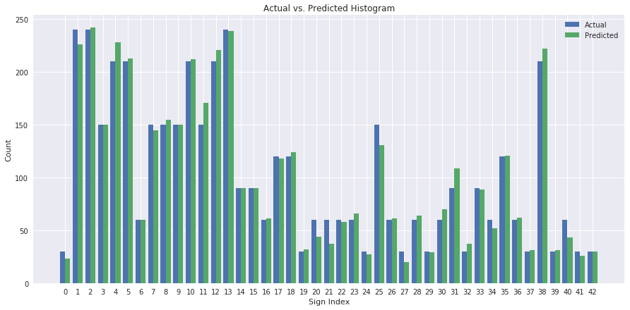
While the model is performing fairly well, we can dive deeper in to the performance of the model to figure out what is happening with the predictions. Specifically, below are the histogram and confusion matrix of validation actuals vs. the validation predicted. By looking at the histogram and confusion matrix, we can look at where the classifications are mistaken and what classes are typically wrong.

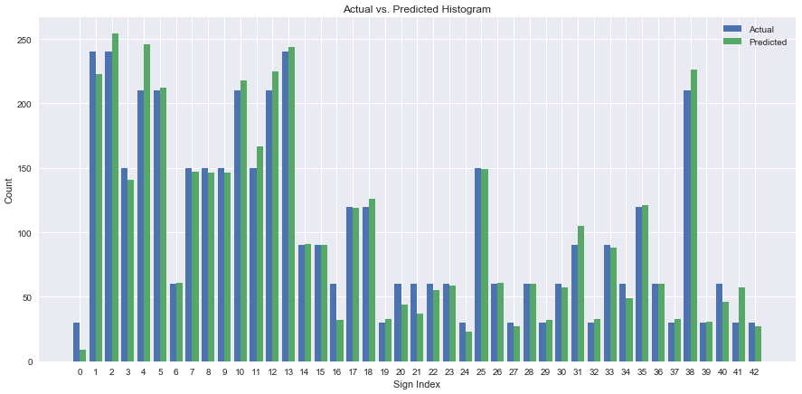
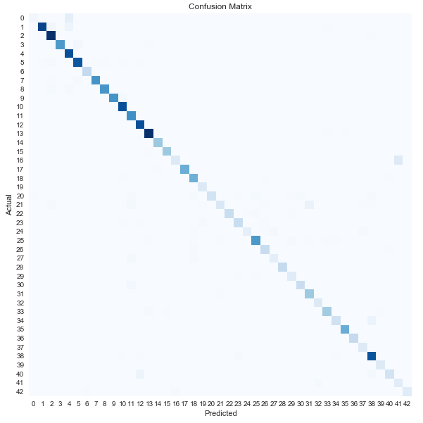
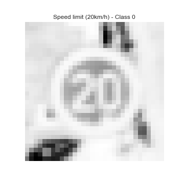
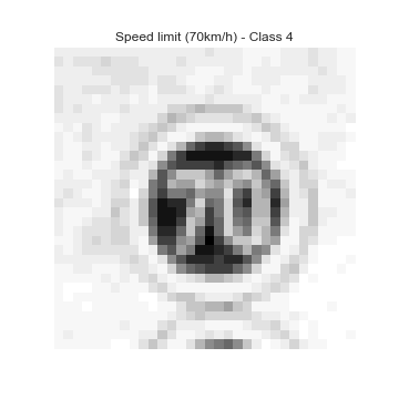
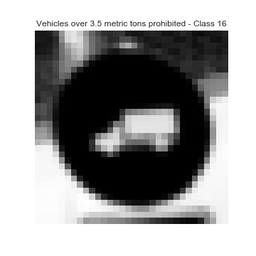
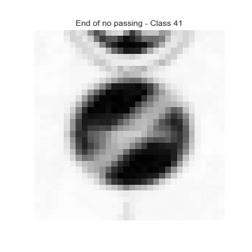
If we look at the histogram above, we see that most of the bars are at about the same place. Similarly, it seems like the diagonal is quite well defined, which means that the CNN did fairly well! However, if we look at the off diagonal cells in the confusion matrix, we see that there are definitely misclassifications. For example, what is actually supposed to be class 0 gets misclassified as class 4 or class 16 gets misclassified as class 41. Below are sample images from these classes.

Class 0 misclassified as Class 4

Class 16 misclassified as Class 41

Data Augmentation

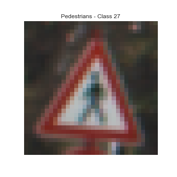
So it seems fairly reasonable, especially for the class 0 to class 4 example for the network to misclassify the images. It even looking at the gray and normalized images the differences between the two are not that drastic. In order to improve the model's performance on these, we can augment the dataset by creating more images with various operations like zooming and rotating the images. Note that it seems like the classes that are more often misclassified are also the classes with the fewest amount of data. This step took an unexpectedly long time because many additional images were created of the under represented classes. With these additional images, I retrained the model. Overall, 11915 additional images were created and a few of the additional images are shown below.

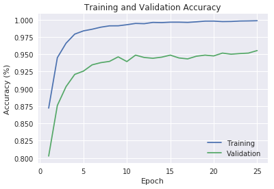
After training with the additional images and increasing the number of epochs to 25, the accuracy on the validation set increased to ~95%. The actual vs. predicted histogram and training/ validation curve also shows an improvement. If we look closely at the actual vs. predicted histogram, it seems like the classes that were misclassified previously are now more accurately classified, which means the data augmentation worked!

Iterative Model Building

As evidenced above, the process of training, validating, and testing the model architecture took an extended amount of time. Mainly because after running the the model over the validation set, I would return to the preprocessing stages to experiment with various other methods for preprocessing.

When fiddling with the model's hyperparameters, I had to switch over to use AWS to train the model because with the additional images and an increased number of epochs, the model was too slow to run on my local machine. Specifically, I launched a g2.2xlarge Amazon EC2 instance and it took ~2-3 minutes to train on the 45,000+ image training set with 25 epochs.

In terms of further improvement on the model, the training and validation curves are still fairly separated meaning the model is still overfitting. In the future, I will consider applying L2 regularization and/or increasing the dropout % to reduce the chance of overfitting.

Design and Test a Model Architecture

In terms of the model architecture that was used to achieve the results above, I used a modified version of the LeNet-5 architecture (shown below). The code used to build the CNN is under the "Model Architecture" section of the Jupyter Notebook.

LeNet Architecture (Actual architecture is slightly different)

Specifically, the model had the following setup:

Layer	Description
Input	32x32x1 Grayscale/ Normalized image
Convolution 5x5	1x1 stride, valid padding, outputs 28x28x6
RELU activation
Max pooling	2x2 stride, valid padding, outputs 14x14x6
Convolution 5x5	1x1 stride, valid padding, outputs 10x10x16
RELU activation
Max pooling	2x2 stride, valid padding, outputs 5x5x16
Fully connected	400 input, 120 output
RELU activation
Dropout	0.6 keep probablility (training)
Fully connected	120 input, 84 output
RELU activation
Dropout	0.6 keep probablility (training)
Fully connected	84 input, 43 output

The above architecture with EPOCHS = 25, BATCH_SIZE = 128, and LEARNING_RATE = 0.001 ended up doing fairly well achieving:

• Training Set Accuracy: ~99.8%
• Validation Set Accuracy: ~95%
• Test Set Accuracy: ~94%

In terms of the optimizer used, I considered using various optimizers such as regular gradient descent, but one of the considerations for switching to the Adam optimizer was that the Adam optimizer takes into account "momentum". Specifically, the Adam optimizer (read more here) takes "momentum" into account by keeping a decaying average of the past gradients, which usually provides quicker convergence.

Test a Model on New Images

In order to further test the model's performance on previously unseen images, I found 6 images from Google Maps Street View to test with the model. Looking at the images below, there are couple factors that might affect the model's ability to classify these new traffic signs. For example, the "Road Work" and "Road Narrows on the Right" signs are captured at an angle. This skew in the image might not get captured by the model because the training data might not have images that are similar. However, when building the training data (via augmenting more images) I tried to include rotated images to deal with this possibility. Additionally, the reduced brightness and skew in the "No Entry" image were potential problems for the classifer.

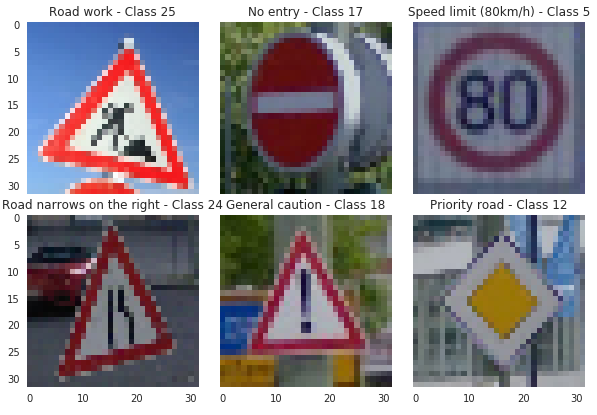
I plotted the top 5 predictions (based on softmax probabilities) for the 6 different images.

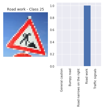
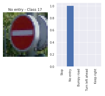
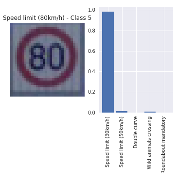
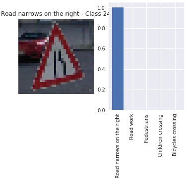
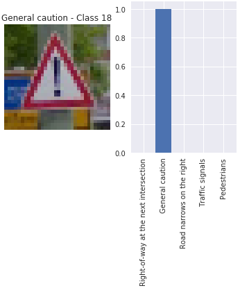
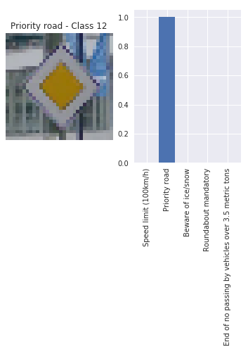
From the results above, it seems like the concerns mentioned were actually handled fairly well by the classifier. Most of the images with the skew and brightness concerns are handled well and the probabilities also show that the model was not "unsure" between classes (except for the 80 kph vs 30 kph sign). The model achieved a ~83.3% accuracy with 5/6 images correctly classified. The 80 kph sign was misclassified as 30 kph, but this is understandable because the model might have mistaken the 8 as a 3. When looking at the image, it seems quite obvious that the image is 80. Ultimately, I may have to add more 80 kph signs with various image translations to ensure the model does not mistakenly classify these signs.

When compared to the test set, the unseen images has a lower accuracy, but it is because of the misclassification mentioned above. On the other images, the model is quite certain (high probability), while for the misclassified image has visible uncertianty (in the bar graphs of the probabilities). Overall, the model seemed to do quite well on unseen data!

Conclusions and Next Steps

This project was quite interesting and gave me the opportunity to learn more about Tensorflow, convolutional neual networks, and how to train, validate, and test a model using an Amazon EC2 instance. Additionally, I got the opportunity to experiment with preprocessing steps to improve the image classification and I learned the importance of augmenting under represented classes.

While the model performed fairly well, there are improvements that can be made.

• Further regularization: Based on the training and validation curves, the model can definitely be further regularized
• Data augmentation: While I experimented with rotation and zooming on images, it may have helped to further translate, crop, and manipulate images to increase the training set and increase the variety of input images
• Hyperparameter tuning: The model performed fairly well but with more time I could have increased the number of epochs or fiddled with the batch size further to see if the model performance improves
• Model architecture: The LeNet architecture is a good start, but with state-of-the-art advancements such as Google's Inception-V3 there are other architectures that might work even better

Ultimately, this was an exciting project that gave me the opportunity to bring together many different techniques and technologies to solve and interesting problem!